In our last article, Inside the Black Box: Developing Explainable AI Models Using SHAP, we discussed the importance of developing explainable AI, exploring techniques that shine a light on the proverbial AI “black box” with the ability to quantify the impact of model input features on a per-outcome basis. Here, we illustrate the application of the SHAP values on various models trained to predict the chances for survival on the RMS Titanic. All Python code is provided in a Jupyter notebook so that you can easily replicate our work.
Explaining a Passenger Survival Model for the RMS Titanic
On April 15, 1912, the RMS Titanic hit an iceberg in the North Atlantic Ocean about 400 miles south of Newfoundland, Canada and sank. Unfortunately, there were not enough lifeboats onboard to accommodate all passengers and 67% of the 2,224 passengers died. Kaggle has an ongoing competition in search of a machine learning model that most accurately predicts the fate of each passenger. As our goal is to explain model decisions via SHAP values, we will not focus on creating the best model possible and will instead examine the output of a variety of models built using their default parameters. Let's start by generating features from Titanic data as provided by Kaggle for training an AI model.
passenger_id: Passenger identifier (used only as an identifier and not for training)
ticket_class: Class of ticket (1 = 1st class, 2 = 2nd class, 3 = 3rd class).
num_family: Number of family members accompanying each passenger.
deck: Deck level, parsed from the original cabin number in original data and with a deck level mapping: (A = 1, B = 2, C = 3, D = 4, E = 5, F = 6, G = 7, U = 8). Note that 77.1% of the cabin numbers were missing and so a vast majority were assigned to deck level U:8, representing unknown.
age: Passenger age, imputed from a random forest model when missing using other features in the data set.
emb_C, emb_Q, emb_S: Port of Embarkation C = Cherbourg, Q = Queenstown, S = Southampton. These are one-hot-encodings of the embarkment feature.
ticket_price: Ticket price.
is_female: Logical variable indicating female or not (0 = no, 1 = yes).
title: Replaced with coded map of titles: (Mr = 1, Miss = 2, Mrs = 3, Master = 4, <RARE> = 5}, where <RARE> titles are Lady, Countess, Capt, Col, Don, Dr, Major, Rev, Sir, Jonkheer, Dona, i.e., those passengers with relatively rare status titles.
survived: Target variable (0 = did not survive, 1 = survived).
surname_length, random: Number of characters in passenger surname and a randomly drawn integer. These variables are added to test the SHAP algorithm: they should not be viewed as important relative to other features in the training data.
You may have noticed that the categorical features, such as deck level, passenger title, and port of embarkation were converted to coded integers, which is often a requirement of many machine learning algorithms. Some algorithms handle such coding "behind the scenes" but here we do so explicitly to make clear the range of values for each feature. With these features formed, can we gain any insight into what features may be important for prediction? One simple way to do so is to investigate the distributions of the data against the target variable.

Figure 1: Histograms of various training features provide basic insight into the data and suggest features that are likely to be important. For example, age plays an important role in deciding a passengers fate with kids mostly surviving and the elderly mostly dying. The counts for the survival classes are stacked, i.e., the no counts do not occlude the yes counts and vice versa.
Figure 1 shows histograms for select features grouped by survival. Beside the plots, the distributional characteristics are briefly discussed with the takeaway that title, deck, age, and ticket_class intuitively are important predictors of passenger fate. Armed with these insights,
our goal is to train a model and calculate the SHAP values for select predicted outcomes (i.e. specific passengers), which will reveal the features seen as important to a model in forming its decision for these specific cases.
As a reminder, SHAP values have the following properties and interpretations:
A SHAP value is generated for each feature and for every predicted outcome.
The magnitude (absolute value) of a SHAP value is proportional to the importance of the corresponding feature.
SHAP values for a given decision are additive and explain how a given outcome f(x) can be obtained relative to an average (baseline) outcome. Expressed mathematically, f(x) = baseline + SHAP[1] + SHAP[2] + … + SHAP[N], where N is the number of features in our training data.
SHAP values are estimated relative to a baseline, which in our case is the average predicted outcome for all passengers in the training data. In the literature, this average training data outcome is referred to as a naive estimator and qualitatively represents a good guess of an arbitrary passenger's fate if we knew nothing about them. SHAP values thus define how a given passenger is "special" relative to the average passenger in our Titanic study.
SHAP values can be negative, positive, or zero. In our study, positive means a better chance of survival, which we discuss below, and so a positive SHAP value means that the corresponding feature bettered the chance of survival for a passenger relative to the average passenger. A negative value means the corresponding feature lessened that passenger's chances for survival relative to the average passenger.
It is important to note that SHAP values are generally sensitive to the corresponding feature value. For example, we see in Fig. 1 that the age feature is important in deciding a passenger's fate. However, a passenger who is 70 years old (likely to die) is different from a passenger who is 5 years old (likely to live). This sensitivity should be reflected by the SHAP value. Specifically, we expect a negative age-SHAP value for a passenger who is 70 and a positive age-SHAP value for a passenger who is 5. An age-SHAP value for a 30 year old is likely to be closer to zero.
Please see our article, Inside the Black Box: Developing Explainable AI Models Using SHAP, for more details on the interpretation of SHAP values and how they are calculated.
Now it's time to build a model. As we aren't particularly interested in assessing model efficacy at this point (any decent model will do), we won't split our data into test and training sets per usual and just train our model using all available data. Later, when we compare model efficacies, we will split our data into training and test sets accordingly. We choose the popular XGBOOST model as a first go to predict the fate of each passenger, i.e., whether or not the passenger will survive (1) or perish (0). In this case, we use a regression model, which generally does not predict exactly 0 or 1 and instead predicts a real value on the interval [0, 1]. A predicted outcome less than 0.5 means the passenger is predicted to perish while a value greater than 0.5 means the passenger is predicted to survive.
We trained an XGBOOST model, then used the SHAP package to estimate the SHAP values for each prediction. A nice way of visualizing the SHAP values is through so-called additive force layout plots as shown in Figure 2. The plots highlight important features that played a role in moving a given passenger's decision towards or away from the naive/average model prediction. In this case, the average prediction over the training data was 0.4265 and is referenced in the force layout plots as the base value. The predicted outcome for a given passenger is denoted as f(x). To get to f(x), we start at the base value and add up the SHAP values. Due to space constraints, only the important SHAP values are visible in the force layout plots. Let's examine the decisions made for three Titanic passengers, using the SHAP values to gain insight into the model's predicted decision:
Passenger 446 was predicted to have an 80% chance of survival, which is much greater than the average passenger with a baseline survival rate of 42.65%. According to the SHAP values, the dominant reason for passenger 446's predicted survival was that he carried the title=4:master. It helped that he was a very young child traveling with family and quartered on the first deck.
Passenger 80 was predicted to have a 47% chance of survival, slightly better than the baseline average but not positive. The primary positive contributor was having title=2:Miss but that was offset by holding a 3rd class ticket, being close to the mean age of all passengers, and being quartered on deck 8.
Passenger 615 was predicted to have a dismal 23% chance of survival, driven primarily by the fact that he was a title=1:Mr. Being quartered on deck 8 did not help and holding a 3rd class ticket while being close to the average passenger age also worsened his chances for survival.

Figure 2: Explanations for the predicted outcomes of three passengers. The features x for each passenger are displayed followed by an additive force layout, which graphically conveys prominent SHAP values that influenced each decision. The term f(x) is the evaluation of the trained model f on the features x, which is the predicted outcome for the corresponding passenger. The base value (= 0.4265) serves as a reference for the force bars, and is calculated as the average predicted outcome over the training data. Red (blue) force bars represent features that have increased (decreased) the passengers chance for survival, relative to the base value. The wider the force bars are, the more influential the corresponding feature.
To get an overview of which features are most important in our model, we can plot the SHAP values of every feature for every passenger (see Figure 3).

Figure 3: SHAP values for top features for every passenger in the training data. For each feature, the associated SHAP value is plotted on the x-axis. Each point represents a single model decision. The more influential a feature is, the more negative or positive it's associated SHAP value. A SHAP value of 0 means that feature did nothing to move the decision away from the naive/reference value. In the plot, we see that the title feature is highly influential with strong negative and positive SHAP values for many predicted outcomes. The color of the points has to do with the relative scaling of the feature values. For example, notice the light blue blob of the title predictions, centered around SHAP values between -0.2 and -0.1. The blue color means that those title values are relatively low, as is the case for Mr = 1. Thus, having a title of Mr has a strong negative impact on your chances of survival, which aligns with our intuition as gathered by the distributions shown in Fig. 1. Similarly, high deck values decrease a passenger's chance of survival (red clump on deck row). This too is what we intuited with deck level assignment U = 8 in Fig. 1.
Finally, we can summarize overall feature importance by calculating the mean absolute value of the SHAP values for each feature (see Figure 4). The features that are estimated to be important (such as title and ticket_class) are intuitive, particularly based on the distributions that we observed in Fig. 1. The other features that we naturally would consider non-impactful, e.g., random, embarkment site and surname length, have relatively small SHAP values. These findings give us confidence in the underlying methodology.

Figure 4: Model feature importance ranked by mean absolute SHAP. This plot shows how important each feature was on average over the passenger population.
SHAP value consistency across models
Generally, you should expect that the features seen as important in one model type are not necessarily seen as important in another model type. However, observing consistency between model types is helpful in trusting and interpreting the resulting SHAP values. To that end, we ran an experiment where we trained several different classification models and ranked the top five features based on mean absolute SHAP value. The models we built were tree-based (DecisionTree, RandomForest, XGBOOST), neural network (multilayer perceptron), and logistic regression. We trained each model using 80% of the labeled Titanic data and tested the model accuracy with the remaining 20%. The top five features for each classifier is shown in Table 1 along with the test accuracy.
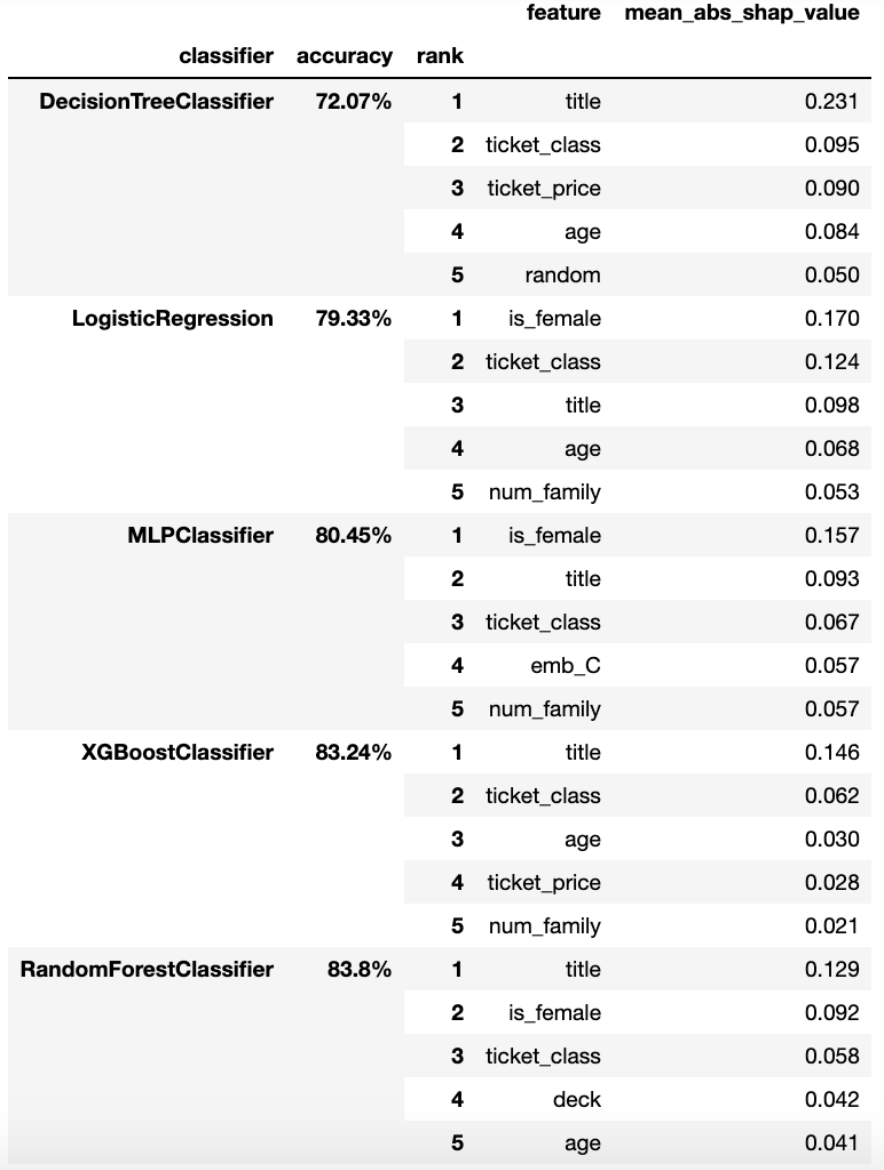
Table 1: Comparison of the top five features, ranked first by model test accuracy and then by the mean absolute SHAP value.
The comparison reveals that a few features are consistently impactful across model types (e.g., title, ticket_class, and age) while the impact of other features is more or less model dependent. As a simple gauge of importance across all models, we formed a weighted sum of the mean absolute SHAP values shown in Table 1 and then normalized by the maximum result to yield cross-model importance ranging from 0 (not important) to 1 (very important). The weights used in the summation were chosen to be the model accuracies so that models that performed better had more influence. Figure 5 shows the cross-model importance for all features.

Figure 5: Estimate of the importance of each feature using the output of all models.
Summary
Many AI models are highly complex and consequently their predicted outcomes are difficult to explain. Recent advancements have been made in understanding complex models by quantifying the influence of features on a per-outcome basis. In this article, we explored one such approach, known as the SHAP values, and demonstrated their use on various AI models trained to predict the fate of each passenger on the RMS Titanic. SHAP values and similar approaches help to shine a light on the proverbial "black box" label given to AI, where inputs are fed into a model where "magic" happens and predictions are made. With SHAP values, we now have the ability to explain why a model made a given decision, which is of considerable importance in gaining insight into training data as well as the inner workings of a model.